Fluid-structure interaction (FSI) problems play a crucial role in many engineering applications, particularly in the nuclear industry, where internal components such as fuel rods and steam generator tubes are subjected to fluid-induced vibrations. These vibrations can lead to structural fatigue, wear and, in extreme cases, the failure of critical components.

The Arbitrary Lagrangian-Eulerian method

To determine the flow of a fluid, one can adopt either an Euler description (a fluid particle identified by its instantaneous position) or a Lagrange description (identified by its initial position). Both lead to forms of the Navier-Stokes equations discretized on a stationary mesh (Euler) or a mesh that follows the fluid particles (Lagrange); in both cases the mesh does not account for the motion of the boundaries. To overcome this, the Arbitrary Lagrangian-Eulerian (ALE) method [37], [58], [97] is used (immersed boundary methods [139], [141], [140] are another option).

ALE kinematic description

In the ALE approach, the fluid flow is computed in a domain deformed to follow the fluid-solid interface. The computational mesh moves with an arbitrary velocity $\boldsymbol{v}_{ALE}$, independent of the material motion: it is zero in the Eulerian approach and equal to the fluid velocity in the Lagrangian approach, and varies smoothly between them in the ALE method (Lagrangian near solids, Eulerian elsewhere). Neither the Lagrangian (material) configuration $R_{\mathbf{X}}$ nor the Eulerian (spatial) configuration $R_{\mathbf{x}}$ is taken as reference; a third referential (ALE) configuration $R_{\boldsymbol{\xi}}$ with mixed coordinates $\boldsymbol{\xi}$ identifies the grid points [37]. The referential domain is mapped into the material domain by $\mathbf{\Psi}$ and into the spatial domain by $\mathbf{\Phi}$.

Lagrangian \f$\mathbf{X}\f$, Eulerian \f$\mathbf{x}\f$ and ALE \f$\boldsymbol{\xi}\f$ frame references and the transformations relating them.

The mapping $\mathbf{\Psi}^{-1}:(\mathbf{X},t)\mapsto(\boldsymbol{\xi},t)$ has gradient

\[\frac{\partial \mathbf{\Psi}^{-1}}{\partial (\mathbf{X}, t)} = \begin{pmatrix} \dfrac{\partial \boldsymbol{\xi}}{\partial \mathbf{X}} & \boldsymbol{v}_{ALE}\\ \mathbf{0}^{T} & 1 \end{pmatrix}, \qquad \boldsymbol{v}_{ALE}(\mathbf{X},t)=\left.\frac{\partial\boldsymbol{\xi}}{\partial t}\right|_{\mathbf{X}} \]

The Jacobian $J(\mathbf{X},t)=\det(\left.\frac{\partial\boldsymbol{\xi}}{\partial\mathbf{X}}\right|_t)$ relates the volume elements ( $dV=J\,dV_0$) and satisfies [36] $\left.\frac{\partial J}{\partial t}\right|_{\mathbf{X}}=J\,\nabla\cdot\boldsymbol{v}_{ALE}$.

ALE form of the governing equations

Relating the material and referential time derivatives gives the fundamental ALE relation $\left.\frac{\partial f}{\partial t}\right|_{\mathbf{X}}=\left.\frac{\partial f^*}{\partial t}\right|_{\boldsymbol{\xi}}+\boldsymbol{v}_{ALE}\frac{\partial f^*}{\partial\boldsymbol{\xi}}$, and, applied to the Navier-Stokes equations, the local form in a frame moving at $\boldsymbol{v}_{ALE}$:

\[\left\{\begin{aligned} \left.\frac{\partial (J \boldsymbol{v})}{\partial t}\right|_{\mathbf{X}} &= J\left(\nu\Delta\boldsymbol{v}-\nabla\cdot(\boldsymbol{v}\otimes(\boldsymbol{v}-\boldsymbol{v}_{ALE}))-\frac{1}{\rho}\nabla p\right),\\ \nabla\cdot\boldsymbol{v} &= 0. \end{aligned}\right. \]

The transport velocity is modified by the grid velocity; the Lagrangian ( $\mathbf{\Psi}=\mathbf{I}$, $\boldsymbol{v}=\boldsymbol{v}_{ALE}$) and Eulerian ( $\mathbf{\Phi}=\mathbf{I}$, $\boldsymbol{v}_{ALE}=\mathbf{0}$) descriptions are contained as particular cases.

Grid motion

The arbitrary mesh velocity must keep the mesh motion under control. In general a new elasticity equation is solved; for moderate deformations, a variable-diffusivity Laplace problem (an extension of the classical harmonic mesh motion [39]) is posed:

\[\left\{\begin{aligned} \nabla\cdot(\mu\,\nabla\boldsymbol{v}_{ALE}) &= \mathbf{0} && \text{in the fluid domain,}\\ \boldsymbol{v}_{ALE} &= \boldsymbol{v}_{S} && \text{at a solid interface,}\\ \boldsymbol{v}_{ALE} &= \mathbf{0} && \text{at a free surface,} \end{aligned}\right. \]

with a spatially varying diffusivity $\mu(K)=\frac{1}{|K|}$ (cell volume), which makes smaller cells stiffer and concentrates the deformation in larger cells away from walls (the classical harmonic case is $\mu=1$). The mesh is updated as $\mathbf{x}^{new}=\mathbf{x}^{old}+\Delta t\,\boldsymbol{v}_{ALE}$.

Finite-volume ALE formulation and velocity-pressure coupling

In the ALE approach the Navier-Stokes equations are naturally written in conservative form over a time-dependent control volume $K(t)$:

\[\frac{d}{dt}\int_{K(t)}\boldsymbol{v}\,d\boldsymbol{x}=\int_{K(t)}\left(\nu\Delta\boldsymbol{v}-\nabla\cdot(\boldsymbol{v}\otimes(\boldsymbol{v}-\boldsymbol{v}_{ALE}))-\frac{1}{\rho}\nabla p\right)d\boldsymbol{x},\qquad \int_{K(t)}\nabla\cdot\boldsymbol{v}\,d\boldsymbol{x}=0 \]

with the transport (relative) velocity $\boldsymbol{w}=\boldsymbol{v}-\boldsymbol{v}_{ALE}$. A finite-volume discretization interprets the discrete velocity $\boldsymbol{v}_K$ as a cell average, approximates the conservative time derivative by $\frac{V_K^{n+1}\boldsymbol{v}_K^{n+1}-V_K^{n}\boldsymbol{v}_K^{n}}{\Delta t}$ (with $V_K=|K(t)|$ the cell volume), and writes the spatial operators as face flux balances.

Note: Remark on the former Jacobian-based implementation. Earlier versions of TrioCFD wrote the ALE equations using the Jacobian $J$ (appearing in the time derivative and all spatial operators), requiring the explicit computation of $J=\det(\partial\boldsymbol{x}/\partial\boldsymbol{\xi})$. The current implementation replaces this by the volume-based finite-volume formulation: at the continuous level the two are equivalent (the factor $J$ is a change of measure), but absorbing the change of variables into the geometric quantities (cell volumes, face areas and normals) avoids the fragile computation of $J$ on distorted cells, is consistent with the cell-average interpretation, and satisfies the Geometric Conservation Law (GCL) by construction. The ALE options and input data are unchanged for the user.

After time discretization with an implicit Euler scheme, the semi-discrete system is

\[\left\{\begin{aligned} \frac{M^{n+1}U^{n+1}-M^{n}U^{n}}{\Delta t} &= A^{n+1}U^{n+1}-L^{n+1}(W^{n})U^{n+1}-(B^{n+1})^{T}P^{n+1}+S^{n+1},\\ B^{n+1}U^{n+1} &= 0, \end{aligned}\right. \]

where $M^{n}$, $M^{n+1}$ are diagonal mass matrices ( $(M)_{KK}=V_K$), $A^{n+1}$ the (symmetric, negative semi-definite) diffusion operator, $L^{n+1}(W^{n})$ the (non-symmetric) convection operator depending on the relative velocity $W^{n}=U^{n}-U_{ALE}^{n}$ (frozen in time), $B^{n+1}$ the discrete divergence operator and $(B^{n+1})^{T}$ its adjoint (the pressure gradient), and $S^{n+1}$ the volumetric source terms (multiplied by the cell volume).

The coupled system is solved by a prediction-correction velocity-pressure splitting:

Velocity prediction: $\left(\frac{1}{\Delta t}M^{n+1}-A^{n+1}+L^{n+1}(W^n)\right)U^{*}=\frac{1}{\Delta t}M^{n}U^n-(B^{n+1})^{T}P^n+S^{n+1}$.
Pressure correction: $B^{n+1}(M^{n+1})^{-1}(B^{n+1})^T P'=\frac{1}{\Delta t}B^{n+1}U^*$.
Velocity correction and pressure update: $U^{n+1}=U^{*}-\Delta t(M^{n+1})^{-1}(B^{n+1})^T P'$, $P^{n+1}=P^n+P'$.

This preserves the conservative character of the ALE finite-volume formulation and accounts for mesh motion through the time evolution of the cell volumes and face geometries.

Large-scale grid motion for ALE

Handling large boundary displacements is a significant limitation of conventional mesh-motion approaches. The proposed strategy first replaces the elliptic formulation by a hyperbolic one (enabling an explicit solution without inverting global systems [107]), then incorporates fictitious material behaviour through the open-source MGIS interface [75] into MFront [74] (see [52]), avoiding the need for application-specific material mechanics code.

Hyperbolic equation for the nonlinear grid problem

The mesh motion is governed by a damped wave-propagation equation (a single damping coefficient $d_g$ suppresses unwanted temporal oscillations, keeping the grid response close to the quasi-static elliptic solution):

\[\rho_g\frac{\partial^2\mathbf{u}_g}{\partial t^2}+d_g\frac{\partial\mathbf{u}_g}{\partial t}-\nabla\cdot\boldsymbol{\sigma}_g[\mathbf{u}_g]=0 \quad \text{in }\Omega_F(t), \]

with $\mathbf{u}_g=\mathbf{u}_{imp}$ on the Lagrangian boundary $\Gamma_{lag}(t)$ and $\boldsymbol{\sigma}_g\cdot\mathbf{n}=0$ on the rest of $\partial\Omega_F(t)$.

The equation is discretized in time by the explicit central-difference (Newmark) scheme [123]; its conditional stability requires the CFL condition $\Delta t_g<\min_{i}\frac{l_i}{c_i}$ [24] ( $l_i$ the characteristic length, $c_i$ the speed of sound in cell $i$). When the grid stable time step is smaller than the fluid one, a subcycling algorithm is used for the grid motion.

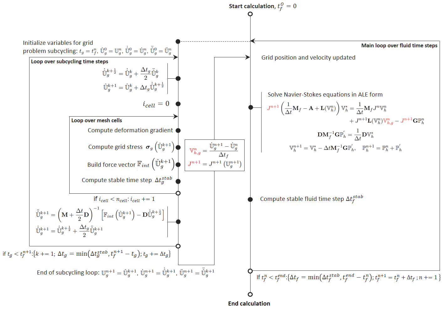
Complete algorithm for the ALE Navier-Stokes solution with the hyperbolic nonlinear problem for mesh motion.

Optimized time-step control and mass scaling

To preserve computational competitiveness, the time-step ratio between the grid and fluid problems should stay below ~200 (and above ~10 to keep a quasi-static grid response) [107]. The fictitious material parameters are chosen first (e.g. $E_g$, $\nu_g$ for the Saint Venant-Kirchhoff model), then the grid density $\rho_g$ is adjusted to set the speed of sound ( $c=\sqrt{E_g/\rho_g}$ for Saint Venant-Kirchhoff). To durably control the ratio, a mass-scaling technique is implemented in the explicit grid solver: for any cell $i$ where $\frac{l_i}{c_i}<\Delta t_g^p$ (the prescribed grid time step), the tangential Young's modulus $E_i^t=c_i^2\rho_i$ (with $\rho_i=\rho_g V_i^0/V_i$) is computed, the requested density $\rho_i^r=E_i^t(\frac{\Delta t_g^p}{l_i})^2$ is matched by adding mass $\delta m_i=V_i\rho_i^r-V_i\rho_i$, distributed among the cell nodes. Since the grid problem does not directly influence the physical fluid solution, mass scaling can be applied safely here.

Material models through MGIS/MFront

MFront provides a Domain-Specific Language to express any constitutive relation, generating and compiling a dynamic library called when the stress is needed; MGIS provides the interface (taking the material library path, parameters including $\rho_g$, and the transformation gradient $\mathbf{F}$, returning the Cauchy stress $\boldsymbol{\sigma}_g$ and the speed of sound $c$). Two models are used for testing: the Saint Venant-Kirchhoff hyperelastic model, and the Ogden hyperelastic model (for nearly incompressible materials at very large strain), with decoupled potential $W(\mathbf{C})=W^v(J)+W^i(\lambda_1,\lambda_2,\lambda_3)$, $W^v=\frac{1}{2}K(J-1)^2$, $W^i=\sum_{p=1}^{N}\frac{\mu_p}{\alpha_p}(\lambda_1^{\alpha_p/2}+\lambda_2^{\alpha_p/2}+\lambda_3^{\alpha_p/2}-3)$, and second Piola-Kirchhoff stress $\mathbf{S}=2\frac{\partial W^v}{\partial\mathbf{C}}+2\frac{\partial W^i}{\partial\mathbf{C}}$. Example input for the Ogden model ( $N=1$):

Structural_dynamic_mesh_model dom
{
  Mfront_library {[local-absolute-path]}{/Ogden/src/libBehaviour.so}
  Mfront_model_name {Ogden}
  Mfront_material_property { {Ogden_alpha}   28.8 }
  Mfront_material_property { {Ogden_mu}   27778.  }
  Mfront_material_property { {Ogden_K} 69444444.  }
  Grid_dt_min 1.e-7
  Density 10000.
  Inertial_Damping 1000.
}

Partitioned coupling with Euler-Bernoulli beams

To reduce the high computational cost of FSI for slender structures, a one-dimensional Euler-Bernoulli beam model is embedded directly within TrioCFD, eliminating code-to-code coupling, 3D interpolation and inter-solver communication. The solid solver uses an unconditionally stable time scheme requiring only diagonal matrix systems; the time coupling follows the explicit Conventional Serial Staggered (CSS) algorithm. The partitioned coupling exchanges variables at the fluid-structure interface $\Gamma_{FS}$, ensuring continuity of the velocities (Dirichlet on the fluid) and of the normal stress (Neumann on the structure):

\[\boldsymbol{v}-\frac{\partial\mathbf{U}}{\partial T}=\mathbf{0}, \qquad (\boldsymbol{\sigma}_f-\boldsymbol{\sigma}_s)\cdot\mathbf{n}_{sf}=\mathbf{0}, \quad \text{on }\Gamma_{FS} \]

Euler-Bernoulli beam model with modal resolution

The structure is modelled by an Euler-Bernoulli beam equation with mass- and stiffness-proportional Rayleigh damping ( $\alpha_1$, $\alpha_2$):

Euler-Bernoulli beam with two bending planes. \f$e_\text{long}\f$ is the beam axis, \f$e_\text{trans,1}\f$ and \f$e_\text{trans,2}\f$ the bending directions, and \f$W_1\f$, \f$W_2\f$ the transverse displacements.

\[\rho_s S\frac{\partial^2 Y}{\partial T^2}+\frac{\partial}{\partial T}\left(2\alpha_1\rho_s S Y+2\alpha_2 EI\frac{\partial^4 Y}{\partial X_1^4}\right)+EI\frac{\partial^4 Y}{\partial X_1^4}=\overline{F} \]

Expanding the displacement on the structural modes $W^{(k)}$, $Y(X_1,T)=\sum_{k=1}^{m}Q^{(k)}(T)\frac{W^{(k)}(X_1)}{N^{(k)}}$, and projecting onto $W^{(l)}$ gives the modal equation $[\mathbf{M}]\ddot{\mathbf{Q}}+[\mathbf{C}]\dot{\mathbf{Q}}+[\mathbf{K}]\mathbf{Q}=\mathbf{F}$, where the mass, damping and stiffness modal matrices are diagonal (modal orthogonality), with $M^{(kk)}=\rho_s S\frac{\langle W^{(k)},W^{(k)}\rangle_L}{(N^{(k)})^2}$, $C^{(kk)}=2(\alpha_1\rho_s S+\alpha_2 EI(\frac{\lambda^{(k)}}{L})^4)\frac{\langle W^{(k)},W^{(k)}\rangle_L}{(N^{(k)})^2}$, $K^{(kk)}=EI(\frac{\lambda^{(k)}}{L})^4\frac{\langle W^{(k)},W^{(k)}\rangle_L}{(N^{(k)})^2}$.

The modal equation is time-discretized with the Hilber-Hughes-Taylor (HHT- $\alpha$) scheme [78], which is unconditionally stable for $\alpha\in[-1/3,0]$, $\beta=(1-\alpha)^2/4$, $\gamma=1/2-\alpha$ ( $\alpha=0$ recovering the Newmark average-acceleration scheme [124]); $\alpha$ introduces high-frequency dissipation. The 3D interface velocity is reconstructed from the modal velocities through the Euler-Bernoulli kinematic relation, and the modal fluid forces are computed by integrating the fluid stress over $\Gamma_{FS}$ (see [102] for details).

Coupling algorithm (CSS)

The explicit Conventional Serial Staggered (CSS) algorithm [136] couples fluid and structure. At time $T^n$, knowing the structure velocity $\dot{\mathbf{U}}^n$, fluid velocity $\boldsymbol{v}^n$ and pressure $P^n$, advancing to $T^{n+1}$ proceeds as:

send the structure velocity $\dot{\mathbf{U}}^{n}$ to the fluid solver;
compute the grid velocity from the harmonic mesh equation with $\boldsymbol{v}_S=\dot{\mathbf{U}}^n$, and update the grid positions;
solve the ALE Navier-Stokes equations for $\boldsymbol{v}^{n+1}$, $P^{n+1}$ with $\dot{\mathbf{U}}=\dot{\mathbf{U}}^n$;
compute the modal fluid forces $\mathbf{F}^{n+1}$ from $\boldsymbol{v}^{n+1}$, $P^{n+1}$ and transfer them to the structure solver;
compute $\ddot{\mathbf{Q}}^{n+1}$, $\dot{\mathbf{Q}}^{n+1}$, $\mathbf{Q}^{n+1}$ via the HHT scheme;
reconstruct the structure velocity $\dot{\mathbf{U}}^{n+1}$;
advance in time (the time step satisfies the fluid CFL condition; the unconditionally stable HHT scheme imposes no solid restriction).

Sketch of the explicit Conventional Serial Staggered (CSS) algorithm. The structure velocity \f$\dot{\mathbf{U}}^{n}\f$ is sent to the fluid solver (1), used to compute the fluid velocity \f$\mathbf{V}^{n+1}\f$ and pressure \f$P^{n+1}\f$ (2); the resulting modal fluid force \f$\mathbf{F}^{n+1}\f$ is transferred to the structure solver (3) and used to update the modal displacement, velocity and acceleration (4).

Beam model configuration

An Euler-Bernoulli beam is configured inside the Beam_model block of a TrioCFD input file (supporting one or two bending planes and an arbitrary beam orientation). Each beam requires modal data (mass/stiffness, mode shapes, abscissae, initial conditions) and geometric/numerical parameters: nb_planes, nb_modes, longitudinal_axis, bendingDirection, BaseCenterCoordinates, NewmarkTimeScheme (MA or HHT), the modal data files (Mass_and_stiffness_file_name, Absc_file_name, CI_file_name, Modal_deformation_file_name), and the Output_position_1D/Output_position_3D output locations. Example (two beams, two bending planes each):

Beam_model dom_cylindres
{
    nb_beam 2
    Name cylindre1 {
        nb_modes 20
        longitudinal_axis z
        bendingDirection x
        nb_planes 2
        BaseCenterCoordinates 0.0035 0. 0.
        NewmarkTimeScheme HHT -0.1
        Mass_and_stiffness_file_name ../Cylindre1/vibr_pout2tube.txt
        Absc_file_name ../Cylindre1/vibr_pout2tube_absc.txt
        CI_file_name ../Cylindre1/vibr_pout2tube_CI.txt
        Modal_deformation_file_name 20 \
            ../Cylindre1/phi_1.txt ../Cylindre1/phi_2.txt ...
        Output_position_1D 1 50
        Output_position_3D 1 0.007 0.0035 0.198
    }
    Name cylindre2 { ... }
}