Phase change and energy conservation

The computation of condensation and evaporation is done in Source_Flux_interfacial_base, which requires a flux_interfacial correlation. When saturation is activated, the total flux is \(\Phi=h_g(T_g-T_{sat})+h_l(T_l-T_{sat})+q_p\) and the relevant latent heat is \(L=\begin{cases}h_l-H_{ls} & \Phi<0\\ h_g-H_{gs} & \text{otherwise}\end{cases}\). If there is no correlation for the phase-change rate \(G\), or if \(|\Phi/L|<|G|\) (limitation by energy conservation), then \(G=\Phi/L\). The phase change \(G\) is further limited by evanescence at \(G_{\text{lim}}\) (see the evanescence treatment in the implementation). The phase enthalpies and their derivatives are switched to the saturated values depending on the sign of \(G\) (so that the donor phase enthalpy is used). These fluxes are distributed to the mass equation (source/sink), the energy equation (heat transfer), and the interfacial-area-concentration equation (condensation/nucleation; see Interfacial Area & Bubble Diameter).

Note: The discrete matrix-filling for these terms ( \(M_\alpha\), \(M_T\), \(M_P\), secmem, and the derivatives \(dG/d\alpha\), \(dG/dT\), \(dG/dP\), with the harmonic mean \(h_m=(1/h_g+1/h_l)^{-1}\) in the energy equation) is given in detail in the source / implementation; only the physical relations are reproduced here.

Interfacial heat flux

The general expression of the interfacial heat flux is \(\phi_{kl}=h_{kl}(T_k-T_l)\). The model (Flux_interfacial_base) fills the exchange-coefficient table hi(k1,k2) and its derivatives with respect to temperature, void fraction and pressure. Most models compute a Nusselt number \(Nu\) and set \(\texttt{hi}(n_l,k)=Nu\frac{\lambda_l}{d_b}\frac{6\max(\alpha_g,a_{min})}{d_b}\), with \(\texttt{hi}(k,n_l)=10^8\) (the gas-side coefficient being very large), and use \(Re_b=\frac{\rho_l d_b(u_g-u_l)}{\mu_l}\), \(Pr=\frac{\mu_l Cp_l}{\lambda_l}\), \(Ja=\frac{\rho_l Cp_l(T_g-T_l)}{\rho_g L_{vap}}\).

Model	Used	Validated	Test case
Constant	Yes	Yes	TrioCFD/CoolProp, TrioCFD/Gabillet, TrioCFD/Canal axi two-phase, Trust/Canal bouillant (two-phase, drift), Trust/Comparaison lois eau
Chen-Mayinger	Yes	No
Kim-Park	Yes	No
Ranz-Marshall	Yes	No
Wolfert	Yes	No
Wolfert composant	Yes	No
Zeitoun	Yes	No

Constant (Flux_interfacial_Coef_Constant): \(\texttt{hi}(k,l)=\texttt{h\_phase}(k)\).
Chen-Mayinger: \(Nu=0.185\,Re_b^{0.7}Pr^{0.5}\).
Kim-Park: \(Nu=0.2575\,Re_b^{0.7}Pr^{-0.4564}Ja^{-0.2043}\).
Ranz-Marshall: \(Nu=2.0+0.6\,Re_b^{0.5}Pr^{0.3}\) (default \(a_{min}=0.01\)).
Wolfert: \(Nu=\frac{12}{\pi}Ja+\frac{2}{\sqrt{\pi}}(1+\nu_t\rho_l\frac{Cp_l}{\lambda_l})Pe^{0.5}\), with \(Pe=\frac{\rho_l Cp_l(u_g-u_l)d}{\lambda_l}\) (default \(Pr_t=0.85\)).
Wolfert composant (to be removed): as Wolfert but with \(\lambda_t=0.06\,Pr_t\,U_\tau D_h\), \(U_\tau=0.1987(u_g-u_l)(\frac{D_h\rho_l(u_g-u_l)}{\mu_l})^{-1/8}\).
Zeitoun: \(Nu=2.04\,Re_b^{0.61}\max(\alpha_g,a_{min,coeff})^{0.328}Ja^{-0.308}\) (with \(Ja=\frac{\max(T_g-T_l,2)\rho_l Cp_l}{\rho_l L_{vap}}\)), with a blending towards \(10^8\) for \(\alpha_g<a_{res}\).

The historic report formulation used the Ranz-Marshall model in the explicit form \(q_{ki}=\frac{6\alpha_v\lambda_l}{d_b^2}\left(2+0.6(\frac{d_b\|\vec{u_l}-\vec{u_v}\|}{\mu_l})^{1/2}(\frac{\mu_l Cp_l}{\lambda_l})^{1/3}\right)(T_v-T_l)\); it has many shortcomings and work is ongoing on better closures.

Wall heat flux

The wall heat flux \(q_{pk}\) is computed by Flux_parietal_base, which fills qpk/qpi (and the nucleation diameter d_nuc) and their derivatives with respect to void fraction, pressure, velocity, fluid temperature and wall temperature.

Model	Used	Validated	Test case
Kommajosyula	Yes	No
Kurul-Podowski	Yes	Yes	TrioCFD/CoolProp

Kommajosyula [96] (to be removed): implemented but dropped, because the original data could not be fitted; not validated. The full Kommajosyula heat-flux-partitioning algorithm (Jakob numbers, departure diameter, bubble growth/wait/boundary-layer times, departure frequency, Hibiki-Ishii nucleation-site density, active-site density, sliding area and surface occupation, split into convection / sliding / evaporation contributions) is documented in the model report and reproduced here for reference:

\[\Phi_{NB}=\underbrace{\Phi_{fc}}_{\text{convection}}+\underbrace{\Phi_{sc}}_{\text{sliding}}+\underbrace{\Phi_{e}}_{\text{evaporation}} \]

with the superheat/subcooling Jakob numbers \(Ja_\text{sup}=\frac{\rho_l Cp_l(T_\text{wall}-T_\text{sat})}{\rho_v L_\text{vap}}\), \(Ja_\text{sub}=\frac{\rho_l Cp_l(T_\text{sat}-T_l)}{\rho_v L_\text{vap}}\), the departure diameter \(d_\text{dep}=18.9\cdot10^{-6}(\frac{\rho_l-\rho_v}{\rho_v})^{0.27}Ja_\text{sup}^{0.75}(1+Ja_\text{sub})^{-0.3}u_l^{-0.26}\), the convection flux \(\Phi_{fc}=(1-S_{sl})h_{fc}(T_\text{wall}-T_\text{liquid})\) (with \(h_{fc}\) from the Kader adaptive wall law [85]), the sliding flux \(\Phi_{sl}=2S_{sl}h_{fc}(T_\text{wall}-T_\text{liquid})\), and the evaporation flux \(\Phi_{e}=\frac{\pi}{6}\rho_v L_\text{vap}d_\text{dep}^3 f_\text{dep}N''_a\).

Kurul-Podowski [100] (depicted in the figure below, from [191]):

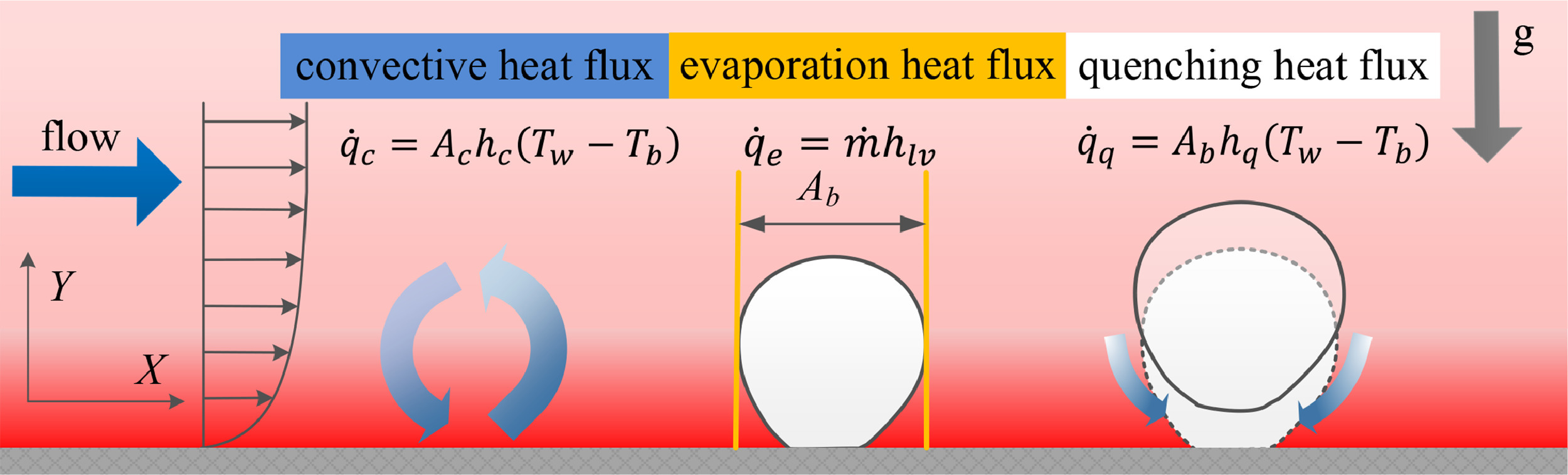
Wall heat-flux partitioning model for subcooled flow boiling (from Zhou 2021).

The single-phase wall heat flux is corrected by the bubble-covered area fraction, \(q_{pk}=q_{pk}^{\text{single phase}}(1-A_{bub})\), and the partitioned (quenching + evaporation) fluxes are added, with:

Evaporation flux \(q_{evap}=f_{dep}\frac{\pi d_b^3}{6}\rho_g L_{vap}N_{sites}\);
Quenching flux \(q_{quench}=A_{bub}\sqrt{f_{dep}}\frac{2\lambda_l(T_p-T_l)}{\sqrt{\pi\lambda_l/(\rho_l Cp_l)}}\);
Number of evaporation sites \(N_{sites}=(210(T_p-T_{sat}))^{1.8}\);
Wall bubble diameter \(d_b=0.0001(T_p-T_{sat})+0.0014\);
Wall bubble total area \(A_{bub}=\min(1,\frac{\pi N_{sites}d_b^2}{4})\);
Departure frequency \(f_{dep}=\sqrt{\frac{4}{3}\frac{9.81(\rho_l-\rho_g)}{\rho_l}}\,d_b^{-0.5}\).

(The corresponding derivatives with respect to the wall temperature, used for the implicit matrix filling, are given in the source.)

Phase change (kinetic limit)

The phase-change mass flux \(G(\alpha,p,T)\) (Changement_phase_base) must be considered when there is a kinetic limit of gas for the phase change — for liquid metals, for example — but it does not apply to water.

Silver-Simpson (Changement_phase_Silver_Simpson, Silver & Simpson 1949): with multiplicative factors \(\lambda_e\) (evaporation), \(\lambda_c\) (condensation), a minimal void fraction \(\texttt{alpha\_min}=0.1\) to activate phase change, and the steam molar mass \(M\), the mass flux is

\[G=\texttt{fac}\times\texttt{var\_ak}\times\texttt{var\_al}\times\texttt{var\_T} \]

with \(\texttt{var\_ak}=\max(\alpha_g,\texttt{alpha\_min})\), \(\texttt{var\_al}=(\max(\alpha_l,\texttt{alpha\_min}))^{1.5}\), \(\texttt{var\_T}=\frac{P_{sat}(T_g)}{\sqrt{T_g+T_0}}-\frac{P}{\sqrt{T_l+T_0}}\), \(\texttt{fac}=\lambda_{ec}\frac{4}{D_h}\sqrt{\frac{M}{2\pi\cdot8.314}}\) and \(T_0=273.15\) K (the \(\lambda_{ec}\) factor selecting evaporation or condensation according to the sign of \(\texttt{var\_T}\)).