|
TrioCFD 1.9.8
TrioCFD documentation
|
|
TrioCFD 1.9.8
TrioCFD documentation
|
A CFD module called CMFD (Computational Multiphase Fluid Dynamics) is under development and is able to handle single- and multi-phase turbulent flows. TrioCMFD uses the PolyMAC_MPFA numerical scheme [66], [65], initially developed for component-scale codes. The resolution of the equations is done using semi-implicit ICE and SETS solvers. Turbulence is treated through two-equation models: an equation on the turbulent kinetic energy \(k\) and one on the turbulent dissipation rate \(\omega\) or time scale \(\tau\). The equations for turbulent quantities are treated like the energy conservation equation and solved in a Newton algorithm in the same matrix as the mass, velocity, pressure and temperature equations. Turbulence acts on the momentum equation through a modified diffusivity (eddy-viscosity hypothesis) and on the energy equation through an SGDH transport term whose Prandtl number the user can tune.
| Variable name | Expression |
|---|---|
| Distance from the face to the element | \(y\) |
| Normal unit vector of the face | \(\overrightarrow{n}\) |
| Velocity at the element centre | \(\overrightarrow{u}\) |
| Perpendicular velocity at the element centre | \(\overrightarrow{u_{\perp}}=u_{\perp}\overrightarrow{n}\) |
| Parallel velocity at the element centre | \(\overrightarrow{u_{\parallel}}=\overrightarrow{u}-(\overrightarrow{u}\cdot\overrightarrow{n})\overrightarrow{n}\) |
| Tangent unit vector | \(\overrightarrow{t}=\overrightarrow{u_{\parallel}}/u_{\parallel}\) |
| Hydraulic diameter | \(D_h\) |
| Dynamic viscosity in the element | \(\mu\) |
| Density in the element | \(\rho\) |
| Kinematic viscosity in the element | \(\nu=\mu/\rho\) |
| Turbulent dynamic viscosity | \(\mu_t\) |
| Turbulent kinematic viscosity | \(\nu_t=\mu_t/\rho\) |
| Dimensionless turbulent kinematic viscosity | \(\nu_{t+}=\nu_t/\nu=\partial_{u_+}y_+-1\) |
| Shear stress at the face | \(\overrightarrow{\tau_f}=-\tau_f\overrightarrow{t}\) |
| Friction velocity | \(u_\tau=\sqrt{\tau_f/\rho}\) |
| Dimensionless distance from face to element | \(y_+=y u_\tau/\nu\) |
| Dimensionless velocity | \(u_+=u_{\parallel}/u_\tau\) |
| Turbulent kinetic energy | \(k\) |
| Dimensionless turbulent kinetic energy | \(k_+=k/u_\tau^2\) |
| Turbulent dissipation frequency | \(\omega\) |
| Dimensionless turbulent dissipation frequency | \(\omega_+=u_\tau^2/\nu\) |
| Turbulent time scale | \(\tau=1/\omega\) |
| Dimensionless turbulent time scale | \(\tau_+=1/\omega_+\) |
| Temperature in the element | \(T\) |
| Temperature in the fluid at the wall | \(T_w\) |
| External temperature (temperature of the wall) | \(T_{\text{ext}}\) |
| Thermal conductivity | \(k_T\) |
| Heat capacity at constant pressure | \(C_p\) |
| Thermal diffusivity | \(\lambda=k_T/(\rho C_p)\) |
| Heat transfer coefficient | \(h\) |
| Heat flux | \(q=h\cdot(T_\text{ext}-T)\) |
| Characteristic temperature | \(T_*=q/(\rho C_p u_\tau)\) |
| Dimensionless temperature difference | \(\theta_+=(T_\text{ext}-T)/T_*\) |
| Prandtl number | \(Pr=\nu/\lambda\) |
| Turbulent Prandtl number | \(Pr_t=\nu_t/\lambda_t\) |
| Von Kármán constant | \(\kappa=0.41\) |
| Liquid fraction | \(\alpha_l\) |
All constants used in the models are user-defined in the calculation dataset, which enables an easy transition from one turbulence model to another.
One of the first models that uses \(\omega\) and not \(\epsilon\) to model the energy dissipation [183]. Here \(\nu_t=\frac{k}{\omega}\). The turbulent equations are:
\[\begin{aligned} \partial_t \rho_l k + \nabla \cdot ( \rho_l k \vec{u_l}) &= \underline{\underline{\tau_R}}:\underline{\underline{\nabla}}\vec{u_l} - \beta_{k}\rho k \omega + \nabla( \rho_l(\nu_l + \sigma_k \nu_t) \underline{\nabla} k) \\ \partial_t \rho_l \omega + \nabla \cdot (\alpha_l \rho_l \omega \vec{u_l}) &= \alpha_{\omega} \frac{\omega}{k}\underline{\underline{\tau_R}}:\underline{\underline{\nabla}}\vec{u_l} - \beta_{\omega}\rho \omega^2 + \nabla( \rho_l(\nu_l + \sigma_{\omega} \nu_t) \underline{\nabla} \omega) \end{aligned} \]
with \(\alpha_{\omega}=0.55\), \(\beta_{k}=0.09\), \(\beta_{\omega}=0.075\), \(\sigma_k=0.5\), \(\sigma_{\omega}=0.5\).
This model [95] was introduced after the Menter SST \(k\)- \(\omega\) model [119], [118] showed the importance of cross-diffusion. The differences with the 1988 Wilcox model are the addition of a cross-diffusion term and a modification of some constants:
\[\begin{aligned} \partial_t \rho_l k + \nabla \cdot ( \rho_l k \vec{u_l}) &= \underline{\underline{\tau_R}}:\underline{\underline{\nabla}}\vec{u_l} - \beta_{k}\rho k \omega + \nabla( \rho_l(\nu_l + \sigma_k \nu_t) \underline{\nabla} k) \\ \partial_t \rho_l \omega + \nabla \cdot (\alpha_l \rho_l \omega \vec{u_l}) &= \alpha_{\omega} \frac{\omega}{k}\underline{\underline{\tau_R}}:\underline{\underline{\nabla}}\vec{u_l} - \beta_{\omega}\rho \omega^2 + \nabla( \rho_l(\nu_l + \sigma_{\omega} \nu_t) \underline{\nabla} \omega) + \sigma_d\frac{\rho_l}{\omega}\max\{\underline{\nabla}k \cdot \underline{\nabla} \omega,\ 0\} \end{aligned} \]
with \(\alpha_{\omega}=0.5\), \(\beta_{k}=0.09\), \(\beta_{\omega}=0.075\), \(\sigma_k=2/3\), \(\sigma_{\omega}=0.5\) and \(\sigma_d=0.5\).
A variation of the 1999 Kok \(k\)- \(\omega\). In this model [94], the time scale \(\tau=\frac{1}{\omega}\) is introduced, so \(\nu_t=k\tau\). An additional diffusion term \(-8\rho_l(\nu_l+\sigma_{\omega}\nu_t)\|\underline{\nabla}\sqrt{\tau}\|^2\) comes out of the calculation:
\[\begin{aligned} \partial_t \rho_l k + \nabla \cdot ( \rho_l k \vec{u_l}) &= \underline{\underline{\tau_R}}:\underline{\underline{\nabla}}\vec{u_l} - \frac{\beta_{k}\rho k}{\tau} + \nabla( \rho_l(\nu_l + \sigma_k \nu_t) \underline{\nabla} k) \\ \partial_t \rho_l \tau + \nabla \cdot ( \rho_l \tau \vec{u_l}) &= - \alpha_{\omega} \frac{\tau}{k}\underline{\underline{\tau_R}}:\underline{\underline{\nabla}}\vec{u_l} + \beta_{\omega}\rho + \nabla( \rho_l(\nu_l + \sigma_{\omega} \nu_t) \underline{\nabla} \tau) \\ &\quad + \sigma_d \rho_l \tau \min\{\underline{\nabla}k \cdot \underline{\nabla} \tau,\ 0\} - 8 \rho_l(\nu_l + \sigma_{\omega} \nu_t) \|\underline{\nabla}\sqrt{\tau}\|^2 \end{aligned} \]
The \(-8\rho_l(\nu_l+\sigma_{\omega}\nu_t)\|\underline{\nabla}\sqrt{\tau}\|^2\) term presents important numerical difficulties close to the wall; three ways of treating it implicitly have been tried, and determining the most robust solution is ongoing. The constants are the same as in the 1999 Kok \(k\)- \(\omega\) model.
The 2006 Wilcox \(k\)- \(\omega\) model [185] is the same as the Kok \(k\)- \(\omega\) with different coefficients (an update of the 1988 Wilcox model). A notable difference is the introduction of a blending function for \(\beta_{\omega}\). The values of the constants are \(\alpha_{\omega}=0.52\), \(\beta_{k}=0.09\), \(\beta_{\omega}=0.0705\cdot f(\Omega_{ij},S_{ij})\), \(\sigma_k=0.6\), \(\sigma_{\omega}=0.5\), \(\sigma_d=0.125\).
At the wall, for elements small enough to be in the viscous regime, the boundary conditions are usually \(\overrightarrow{u}=0\), \(T=T_{\text{wall}}\), \(k=0\), \(\tau=0\), and something smart for \(\omega\) ( \(\omega\rightarrow+\infty\) when \(y\rightarrow0\)). When the first element is too large for the viscous regime to be valid, different boundary conditions must be implemented.
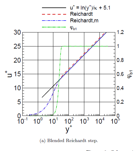
The viscous boundary condition on velocity is \(\overrightarrow{u}=0\). The velocity function used in many codes when the first element is large is the log-law, \(u_{+\text{Log}}=\frac{1}{\kappa}\ln(y_+)+5.1\), valid only for \(30\lesssim y_+\lesssim300\). In 1951, Reichardt [144] proposed a formulation valid for smaller \(y_+\):
\[u_{+\text{Rei}}=\frac{1}{\kappa}\ln(1+0.4y_+)+7.8\left(1-\exp(-y_+/11)-\frac{y_+}{11}\exp(-y_+/3)\right) \]
Here, a blending proposed by Knopp [90] (used in the Fun3D code [15]) is used:
\[\phi=\tanh\left[\left(\frac{y_+}{27}\right)^4\right], \qquad u_+=\phi\, u_{+\text{Log}}+(1-\phi)\, u_{+\text{Rei}} \]
The boundary condition is enforced through the computation of a shear stress, knowing \(u_{\parallel}\) in the first element.
Kalitzin et al. [86] give a complete overview of the possible boundary conditions on \(k\). Inside the viscous sublayer, \(k_{visc}=0\); in the log-law region, \(k_{+,log}=1/\sqrt{\beta_k}\). An often-used proposal is \(\partial_y k=0\). There is no universally accepted blending function. Another proposal uses \(\nu_{t+}=\partial_{u_+}y_+-1\) (not validated in a commercial code), yielding \(k_+=\nu_{t+}\omega_+\) and
\[\partial_y k_+=(\partial_{u_+}y_+-1)\frac{u_\tau^2}{\nu}\partial_y\omega-\frac{u_\tau}{\nu}\frac{\partial_{y_+}^2 u_+}{(\partial_{y_+}u_+)^2}\omega_+ \]
The formulations \(k_{visc}=0\) and \(\partial_y k=0\) are implemented in TrioCMFD. Another simple boundary condition is a home-made transition from the viscous to the zero-flux boundary condition by imposing a flux at the wall:
\[\Phi_{k,\text{wall}}=(\nu_l+\nu_t)/y\cdot(1-\tanh((y_+/20)^2)) \]
Finally, the weak boundary condition above is implemented with an imposed \(k\) flux (see [101] for details on weak wall laws).
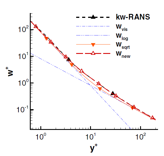
The treatment of \(\omega\) at the wall is one of the difficulties of \(k\)- \(\omega\) models, since \(\omega\rightarrow+\infty\) at the wall. Wilcox recommends inputting the theoretical viscous sub-layer value in the first element, \(\omega_\text{element}=\frac{6\nu}{\beta_\omega y^2}\). Menter [119] recommends at the wall \(\omega_\text{wall}=10\frac{6\nu}{\beta_\omega y^2}\). Knopp [90] proposed a blending function between the viscous and log-law regimes:
\[\phi=\tanh\left[\left(\frac{y_+}{10}\right)^2\right], \quad \omega_{vis}=\frac{6\nu}{\beta_\omega y^2}, \quad \omega_{log}=\frac{u_\tau}{\sqrt{\beta_k}\kappa y} \]
\[\omega_{1}=\omega_{vis}+\omega_{log}, \quad \omega_{2}=(\omega_{vis}^{1.2}+\omega_{log}^{1.2})^{1/1.2}, \quad \omega=\phi\,\omega_{1}+(1-\phi)\,\omega_{2} \]
They also recommend enforcing the theoretical value of \(\omega\) in the first element (as in [15]). The derivative of this theoretical value can also be computed to obtain a flux to input in the first element (the full derivative expression \(\partial_y\omega\) being assembled from \(\partial_y\phi\), \(\partial_y\omega_{vis}\) and \(\partial_y\omega_{log}\)). For now, the only boundary condition implemented is this weak (flux) form, but work is ongoing on others.
The simplest boundary condition is \(\tau_{\text{wall}}=0\) (used in [157]). Another possibility is a weak boundary condition using \(\tau=\frac{1}{\omega}\), giving \(\partial_y\tau=-\frac{\partial_y\omega}{\omega^2}\). Both are implemented; work is ongoing on others.
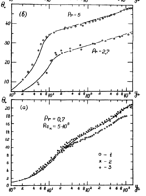
The heat transfer coefficient implemented is the one proposed by Kader [85]. It is compatible with adaptive wall functions, based on experiments and later confirmed by DNS [120]. It is valid in a range \(6\cdot10^{-3}<Pr<6\cdot10^{4}\), for \(Pr_t\approx0.85\):
\[\Gamma=\frac{10^{-2}(Pr\, y_+)^4}{1+5Pr^3 y_+}, \qquad \beta=(3.85Pr^{1/3}-1.3)^2+2.12\ln(Pr) \]
\[\theta_+=Pr\, y_+\exp(-\Gamma)+\left\{2.12\ln\left[(1+y_+)\frac{2.5(2-2y/D_h)}{1+4(1-2y/D_h)^2}\right]+\beta\right\}\exp(-1/\Gamma) \]
In VEF, the turbulence model used is \(k\)- \(\epsilon\). The velocity and the turbulent quantities ( \(k\) and \(\epsilon\)) are vectors located at the centre of the faces. For the velocity equation:
In VEF, the temperature is also located at the faces. To compute the temperature diffusion, TrioCFD uses a separate equation for the turbulence on temperature, recomputing \(u_\tau\), \(k\) and \(\epsilon\) at the boundary faces (usually a Prandtl turbulence model is used to save cost).
See [15]. Compute \(u_\parallel\); compute \(u_\tau\) by Newton's method using \(\frac{u_\parallel}{u_\tau}=u_+(\frac{y u_\tau}{\nu})\); compute the shear stress \(\tau_f=\rho u_\tau^2\); obtain the momentum flux from the wall \(-\tau_f\overrightarrow{t}\); no heat transfer; for the turbulent quantities, it seems \(\omega_{\text{element}}=\omega_{theoretical}\) and \(k_{\text{wall}}=0\) are used (unclear in the paper).
The implementation of shear-induced turbulence for multiphase flows is done by adding the liquid fraction \(\alpha_l\) as a factor in all the conservation equations for the turbulent quantities. For example, the Kok \(k\)- \(\tau\) equations become:
\[\begin{aligned} \partial_t \alpha_l \rho_l k + \nabla \cdot (\alpha_l \rho_l k \vec{u_l}) &= \alpha_l \underline{\underline{\tau_R}}:\underline{\underline{\nabla}}\vec{u_l} - \frac{\beta_{k}\alpha_l\rho k}{\tau} + \nabla(\alpha_l \rho_l(\nu_l + \sigma_k \nu_t) \underline{\nabla} k) \\ \partial_t \alpha_l \rho_l \tau + \nabla \cdot (\alpha_l \rho_l \tau \vec{u_l}) &= - \alpha_{\omega}\alpha_l \frac{\tau}{k}\underline{\underline{\tau_R}}:\underline{\underline{\nabla}}\vec{u_l} + \beta_{\omega}\alpha_l\rho + \nabla(\alpha_l \rho_l(\nu_l + \sigma_{\omega} \nu_t) \underline{\nabla} \tau) \\ &\quad - 8\alpha_l \rho_l(\nu_l + \sigma_{\omega} \nu_t) \|\underline{\nabla}\sqrt{\tau}\|^2 + \sigma_d \alpha_l \rho_l \tau \min\{\underline{\nabla}k \cdot \underline{\nabla} \tau,\ 0\} \end{aligned} \]
The Sato model [155] is implemented in Viscosite_turbulente_sato.cpp. The original formula is
\[\epsilon''=\left(1-\exp\left(-\frac{y^+}{A^+}\right)\right)^2 k_1 \alpha \frac{D_b}{2}U_B \]
with \(A^+=16\) and \(k_1=1.2\). The bubble diameter \(D_b\) is modelled to account for the deformation of the bubble at the wall, and \(U_B\) is the relative velocity. In TrioCFD, the squared coefficient depending on \(y^+\) is not implemented, and the bubble diameter is taken as is without the prescribed function.
The HZDR model [152], [153], [154], [23] adds a production term \(S_{k}^{\text{BI}}\) to the \(k\) equation and a dissipation term \(S_{\omega}^{\text{BI}}\) to the \(\omega\) equation, under the assumption that all energy lost by the bubble to drag is converted to turbulent kinetic energy in its wake [153]. In CMFD, only the production and dissipation terms have been extracted and implemented (without the SST process), so the prescribed coefficient might not be well suited. The two terms are related by
\[S_{\omega}^{\text{BI}}=\frac{1}{C_{\mu}k_l}\mathcal{S}_{\varepsilon}^{\text{BI}}-\frac{\omega_L}{k_L}S_{k}^{\text{BI}}, \qquad \mathcal{S}_{\varepsilon}^{\text{BI}}=C_{\varepsilon B}\frac{S_{k}^{\text{BI}}}{\tau}=C_{\varepsilon B}\frac{S_{k}^{\text{BI}}\varepsilon_l}{k_l} \]
In the code, the dissipation term takes the form \(S_{\omega}^{\text{BI}}=\frac{C_{\varepsilon}}{C_{\nu}D_b\sqrt{k}}\mathcal{S}_{k}^{\text{BI}}\), with
\[\mathcal{S}_{k}^{\text{BI}}=\frac{3}{4}C_k\frac{C_d}{D_b}\frac{\alpha_g}{\alpha_l}u_r^3, \quad C_d=\max\left(\min\left(\frac{16}{Re_b}(1+0.15Re_b^{0.687}),\ \frac{48}{Re_b}\right),\ \frac{8Eo}{3(4+Eo)}\right) \]
\[Eo=\frac{g\|\rho_l-\rho_g\|D_b^2}{\sigma}, \qquad Re_b=\frac{D_b u_r}{\nu_l} \]
By two-phase turbulence we mean the effect of the bubbles on the turbulence in the liquid phase. The models implemented come from the PhD of Antoine du Cluzeau [38]. Following [145], the velocity fluctuations caused by the bubbles are split into wake-induced turbulence (WIT) and wake-induced fluctuations (WIF). The total Reynolds stress tensor is
\[\underline{\underline{\tau_R}}=\underline{\underline{\tau_R}}_{\text{single-phase}}+\underline{\underline{\tau_R}}_{\text{WIF}}+\underline{\underline{\tau_R}}_{\text{WIT}} \]
This model is only available in PolyMAC for now.
Wake-induced fluctuations are the anisotropic effects of the average wake, primarily in the direction of the liquid-gas velocity difference. No transport equation is needed:
\[\underline{\underline{\tau_R}}_{\text{WIF}}=\alpha_v|\overrightarrow{u_v}-\overrightarrow{u_l}|^2\begin{bmatrix}3/20 & 0 & 0 \\ 0 & 3/20 & 0 \\ 0 & 0 & 1/5+3C_v/2\end{bmatrix} \]
with \(C_v=0.36\). A newer formulation (M. El Moatamid, using [10]) gives a tensor for the second part: \(\underline{\underline{\tau_R}}_{\text{WIF}}=\alpha_v\left(\frac{3}{20}u_r^2\underline{\underline{I}}+\left(\frac{1}{20}+0.25\cdot\frac{3}{2}\gamma^3\right)\underline{u_r}\,\underline{u_r}\right)\).
Wake-induced turbulence is the isotropic contribution of bubbles, from the instabilities of the bubble wakes. It takes the form of an additional transport equation for a specific kinetic energy \(k_{WIT}\):
\[\underline{\underline{\tau_R}}_{\text{WIT}}=k^{WIT}\frac{2}{3}\delta_{ij}, \qquad \frac{D k^{WIT}}{Dt}=\underbrace{C_D\nabla^2 k^{WIT}}_\text{Diffusion}-\underbrace{\frac{2\nu_l C_D' Re_b}{C_\Lambda^2 d_b^2}k^{WIT}}_\text{Dissipation}+\underbrace{\alpha_v\frac{\rho_l-\rho_v}{\rho_l}g|\vec{u_v}-\vec{u_l}|\left(0.9-\exp\left(-\frac{Re_b}{Re_b^c}\right)\right)}_\text{Production} \]
where \(C_\Lambda=2.7\), \(Re_b^c=170\), \(C_D'\) is a user-input drag coefficient and \(C_D\) is a turbulent diffusion coefficient. It is implemented in Energie_cinetique_turbulente_WIT.cpp (inheriting from Convection_Diffusion_std); the production, dissipation and turbulent-diffusion terms are modelled by dedicated classes (Production_WIT_PolyMAC_P0, Dissipation_WIT_PolyMAC_P0, Viscosite_turbulente_WIT, and SGDH/GGDH transport models from [3]). To take the WIT into account in the momentum equation, its presence is specified in the diffusion term: