The goal here is to set up a stationary test case. By stationary, we mean that only the stabilized result (i.e. at the end of the transient) is worthy of interest and analysis. In this type of test case, only the final stationary results are correct. The results obtained during the transient period that leads to the final stationary state are not necessarily correct and must not be analyzed.

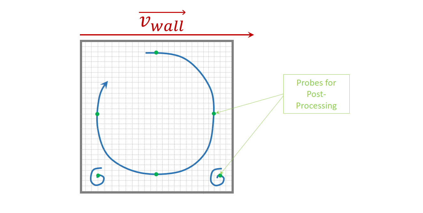
Take the example of a square cavity with a moving top wall (an imposed velocity on the top wall, in single-phase flow). The motion of the top wall creates a main vortex at the center of the cavity, with recirculations at the two lower corners.

Expected stationary state for a flow in a square cavity with a velocity imposed on the top wall

The steps to define this type of computation are as follows:

• The mesh: to correctly account for the imposed velocity of the top wall, it is necessary to define a sufficiently fine mesh at that location. It is also necessary to refine the mesh on the other edges of the domain so that the friction forces are correctly computed. We will therefore define a refined mesh on the edges of the domain and a coarser mesh in its center.
• The physics solved: the problem solved here is a laminar problem, which will be defined with the keyword Pb_thermohydraulique.
• The fluid properties: in the case of an isothermal problem, the fluid properties must be defined at the temperature and pressure of the problem considered (these values are to be found in the state tables).
• The convection scheme: in this case, the choice of the scheme is important. The aim is to find a compromise between a scheme that is too coarse and one that is too fine. If a coarse first-order scheme is used, the small vortices expected in the lower corners of the cavity will be crushed by the numerical viscosity. Conversely, if the scheme is too precise (such as a centered scheme), spurious oscillations may appear. For a VDF discretization, a quick scheme will be preferred, and for VEF a muscl scheme.
• The diffusion scheme: in a stationary laminar case, it is not necessary to define a diffusion scheme.
• The time scheme: to obtain the results of a stationary case, the solver to use is an implicit solver. The objective of this type of computation is to obtain a correct result once the transient has stabilized, not to understand and study the phenomenology of the transient. During the transient period, the results obtained will not necessarily be "correct" and must not be interpreted or analyzed. Only the final results are guaranteed and worthy of interest. We recommend using an implicit Euler scheme with a GMRES scheme for the velocity and a GCP scheme (PETSc conjugate gradients) for the pressure. In the definition of the time scheme, it is recommended to start with dt_min 1e-5. The dt_min has no relation to the physics considered; it simply imposes a minimum time step on the solver in order to avoid time-step drops. It is also recommended to define a printing time step dt_impr = dt_min in order to permanently monitor the computation. The printed output will be visible in the .out and .err output files. It is also recommended to start the computation with a first time step that does not change, in order to have a better initialization (dt_start dt_fixe 1e-3), and to define a safety factor of 10 (fac_sec 10.) which multiplies the convection and diffusion time steps by 10.
• The post-processing: to analyze the results obtained, it is necessary to go through a post-processing block in which we will define probes with a lata output format. These probes must be defined on quantities relevant to the computation considered (here the probes will be on velocity and pressure), but also at locations relevant to the geometry considered. Here the zones of interest are near the walls, but also in the lower corners where recirculation zones will most likely appear. During this dataset-construction phase, it is recommended to define the chosen output frequency as every second.

A first version of the dataset is then assembled and the computation can be launched over 3 seconds, thus providing 3 lata outputs for the various fields defined. It is important to make sure that everything works correctly by first verifying that this preliminary computation finishes properly.

If the preliminary computation does not run, the first reflex is to look at the error message in the .err. If, at this stage, the computation has not succeeded, it is very likely that there is a convergence problem. We then look at the values of the stability time steps, both for convection and diffusion, in the .out output file. If the values of the stability time steps are very small (< dt_min), it is then necessary to decrease the value of dt_min until the computation runs.

If the preliminary computation finishes successfully, we then look at the stability time steps for convection and diffusion in the .out output file in order to adapt the dt of the post-processing (lata) files accordingly. We will rerun the computation over 1000 time steps, having taken care to increase the probe saving frequency to every 100 time steps (versus every second during the preliminary computation). With this new time-step definition, we will obtain 10 probe results (lata) already giving a good impression of the progress of the computation.

If the physical phenomena are still developing, that is, the velocity of each probe has not reached stability, we then increase the computation time (tmax), taking care to adapt the lata frequency accordingly, and we restart the computation. We repeat this step while monitoring the development of the flow through the probes and the lata outputs. We will repeat this step as many times as necessary until the stationary state of the problem is obtained. This stationary state is reached when the evolution of the velocity on all probes becomes constant. By observing the time steps in the .out output file, we notice that TrioCFD progressively increases the time steps because it knows — from the time scheme defined — that the solution sought is a stationary solution, and therefore goes faster and faster to reach this state.

In order to make sure that this stationary state has been reached, it is recommended to look at the residuals. These (accessible in the .out output file) must decrease for the pressure and the velocity.

Warning

Sometimes this decrease does not occur, and may come either from the presence of small vortices that have developed in the flow, or from a poor resolution of one or several cells of the domain.

Typically, in the case considered here, particular attention should be paid to the cell in the upper-right corner of the domain, because it is the meeting point between a fixed wall and the moving top wall. It is then appropriate to determine where these residuals come from and how they stabilize. In this example, they will therefore be purely numerical and will not necessarily mean that there is a physical problem.