|
TrioCFD 1.9.8
TrioCFD documentation
|
|
TrioCFD 1.9.8
TrioCFD documentation
|
The IJK module in TrioCFD relies on the Front-Tracking discontinu module for all the FT mesh management. IJK (a reference to the three components of a Cartesian coordinate system) is optimized for direct numerical simulations in parallelepipedic domains, discretized on a structured Cartesian grid. Its simplified vectorization allows significant performance gains, in particular thanks to the multigrid solver for the resolution of the pressure. This module is used to perform channel flow calculations (wall boundary conditions available in the z direction), as well as periodic calculations. The periodicity for the Front-Tracking interfaces is ensured with a specific algorithm and allows the study of stationary states. The IJK Front-Tracking module is mature for adiabatic calculations of bubbly flows. It is specially designed for bubbly flow studies (neither free surfaces nor droplets) at low void fraction (<10%). To date, there is no model for fragmentation, coalescence or wall boiling.
The Front-Tracking IJK module solves the one-fluid equations of [88] as written for channel up-flow by [111]. Following the proposal of Tryggvason, a front-tracking method is used to solve the set of equations in the whole computational domain, including both the gas and liquid phases. The interface is followed by connected marker points. The Lagrangian markers are advected by the velocity field interpolated from the Eulerian grid. In order to preserve the mesh quality and to limit the need for a smoothing algorithm, only the normal component of the velocity field is used in the marker transport. After transport, the front is used to update the phase indicator function, the density and the viscosity at each Eulerian grid point. The Navier–Stokes equations are then solved by a projection method [138] using fourth-order central differentiation for the evaluation of the convective and diffusive terms on a fixed, staggered Cartesian grid. Fractional time stepping leads to a third-order Runge–Kutta scheme [186]. In the two-step prediction–correction algorithm, a surface-tension source is added to the main flow source term and to the evaluation of the convection and diffusion operators in order to obtain the predicted velocity (see [116]). Then, an elliptic pressure equation is solved by an algebraic multigrid method to impose a divergence-free velocity field.
The shear-periodicity condition consists in imposing on the boundary \(\partial\omega_z\) a periodicity condition accompanied by a velocity jump. To impose a mean linear sheared flow \(U(z)=Sz\) [168], [169], [148], the velocity jump at the boundary \(\partial\omega_z\) is \([\![U]\!]_{\partial\omega_z}=SL_z\). Integrating this jump condition in time gives the spatial shift \([\![X]\!]_{\partial\omega_z}=SL_zt\). Thus, the tri-periodicity of a domain (with shear-periodicity condition along \(z\)) is written:
\[\begin{aligned} \phi(x+L_x,y,z)&=\phi(x,y,z)\\ \phi(x,y+L_y,z)&=\phi(x,y,z)\\ \phi(x,y,z+L_z)&=\phi(x-StL_z,y,z)+[\![\phi]\!]_{\partial\omega_z} \end{aligned} \]
where \(\phi\) represents any variable of the problem (velocity, pressure, density, etc.). Note that \([\![\phi]\!]_{\partial\omega_z}=0\) for all quantities except the velocity.
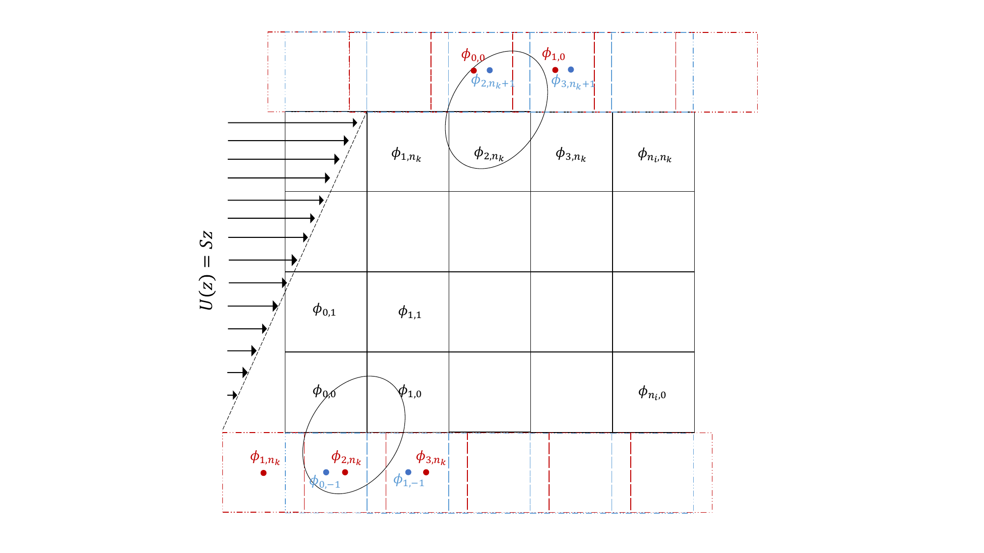
The shear-periodicity condition requires numerous interpolations at the boundary \(\partial\omega_z\), and errors can occur and considerably degrade the computations if they are not handled correctly. For any quantity, an interpolation can be written (with \(i'=i\%n_i\) to account for the periodicity along \(x\); the \(i'\) notation is dropped below for readability):
\[\begin{aligned} \phi_{i,n_k+1}&=\sum_{j\in n_i} a_j(t)\,\phi_{i-j,0}\\ \phi_{i,-1}&=\sum_{j\in n_{i}}a_j(t)\,\phi_{i+j,n_k} \end{aligned} \]
The coefficients \(a_j\) depend on the chosen interpolation (linear regression, higher-order interpolation, etc.). Since the spatial shift is a function of time, these coefficients change at each time step to satisfy the shear-periodicity condition and verify \(\sum_{j\in n_{i}} a_j(t)=1\).
In a two-phase cell, the main flow quantities are solved in one-fluid form, \(\phi=\sum_{k\in[l,v]}\phi_kI_k\), where \(I_k\) is the phase indicator equal to 1 in phase \(k\) and varying between 0 and 1 in two-phase cells. The interpolation of a one-fluid quantity is then:
\[\phi^{i,n_k+1}=\sum_{j\in n_{i}} a_j(t)\left(\phi^{i-j,0}_v I^{i,n_k+1}_v+\phi^{i-j,0}_l I^{i,n_k+1}_l\right) \neq \sum_{j\in n_{i}} a_j(t)\,\phi_{i-j,0} \]
Numerically, the phase indicator function and the exact curvature are known at each instant (including in the "ghost" cells), because TrioIJK uses an extended domain to manage the periodicity of the interfaces. However, for one-fluid quantities a non-trivial interpolation is required: the phasic quantities \(\phi_v\) and \(\phi_l\) are unknown (except for the physical properties when they are constant per phase). This is all the more important for variables presenting a jump at the interface (pressure, density, viscosity).
For thermodynamic properties that are constant per phase, the reconstruction of the one-fluid quantity is trivial once the indicator function is known in the ghost cells:
\[\begin{aligned} \rho_{i,n_k+1}&=\rho_l I^l_{i,n_k+1}+\rho_v I^v_{i,n_k+1}, &\quad \rho_{i,-1} &= \rho_l I^l_{i,-1}+\rho_v I^v_{i,-1}\\ \mu_{i,n_k+1}&=\mu_l I^l_{i,n_k+1}+\mu_v I^v_{i,n_k+1}, &\quad \mu_{i,-1} &= \mu_l I^l_{i,-1}+\mu_v I^v_{i,-1} \end{aligned} \]
For adiabatic conditions, the velocity has no jump at the liquid/vapour interface. Nevertheless, interpolating \(\rho\) and \(\mathbf{U}\) separately does not ensure momentum conservation \(\rho\mathbf{U}\). Two methods are therefore tested:
\[U_{i,n_k+1}=\sum_{j\in n_i} a_j(t)\,U_{i-j,0}+[\![U]\!]_{\partial\omega_z}, \qquad U_{i,-1}=\sum_{j\in n_{i}}a_j(t)\,U_{i+j,n_k}-[\![U]\!]_{\partial\omega_z} \]
\[U_{i,n_k+1}=\frac{1}{\rho_{i,n_k+1}}\sum_{j\in n_i} a_j(t)\,[\rho U]_{i-j,0}+[\![U]\!]_{\partial\omega_z}, \qquad U_{i,-1}=\frac{1}{\rho_{i,-1}}\sum_{j\in n_{i}}a_j(t)\,[\rho U]_{i+j,n_k}-[\![U]\!]_{\partial\omega_z} \]
For the pressure (not constant per phase and presenting a jump at the interface), the situation is more complex. Using the stress-jump relation at the interface in the normal direction, \(P_v^{I}-P_l^{I}+(\tau_{l,n}-\tau_{v,n})=\sigma\kappa^{i,n_k+1}\), where \(\tau_{l,n}\) and \(\tau_{v,n}\) are the deviatoric parts of the stress tensor projected along the interface normal ( \(\tau_{l,n} = \mu_l\nabla\mathbf{u_l}\cdot\mathbf{n^I}\)), and expressing it at first order at the elements, one obtains for the one-fluid pressure interpolation:
\[\begin{aligned} P^{i,n_k+1}=& \sum_{j\in n_{i}} a_j(t)\,P^{i-j,0}+ \sum_{j\in n_{i}} a_j \left[\sigma\left(I_l^{i-j, 0}\kappa^{i-j,0}-I_l^{i, n_k+1}\kappa^{i,n_k+1}\right)\right]\\ &+\sum_{j\in n_{i}} a_j \left[I_l^{i-j, 0}\left(\tau_{v,n}^{i-j,0}-\tau_{l,n}^{i-j,0}\right)-I_l^{i, n_k+1}\left(\tau_{v,n}^{i, n_k+1}-\tau_{l,n}^{i, n_k+1}\right)\right]+O(x_I-x) \end{aligned} \]
The first term of the right-hand side is a classical interpolation of the one-fluid quantity and does not require reconstructing the phasic quantities. The second term expresses the error made when interpolating one-fluid quantities directly (due to the linear interpolation of the phase indicator and curvature) and can be computed numerically, correcting the most important error on the pressure interpolation in two-phase cells. The third term is the contribution of the viscous stress jump at the interface, which should be small compared to the surface-tension jump; since \(\tau_l\) and \(\tau_v\) are not known from the resolution, this term is neglected in the following. The last term \(O(x_I-x)\) is the contribution to the interpolation error related to the offset between the pressure resolved at the elements and the interfacial pressures. In the following, the naive interpolation is used:
\[P^{i,n_k+1}\approx \sum_{j\in n_{i}} a_j(t)\,P^{i-j,0}, \qquad P^{i,-1}\approx \sum_{j\in n_{i}} a_j(t)\,P^{i+j,n_k} \]
In TrioIJK, a Poisson equation of the form \(\nabla\cdot\left(\frac{1}{\rho}\nabla P\right) = f\) must be solved. The discretization of the term inside the divergence is done at the faces, with an arithmetic (or harmonic) interpolation of the density. With the arithmetic mean, the discretization of the divergence operator at the elements gives, in 2D:
\[\alpha_{i+1,k}P_{i+1,k}+\alpha_{i,k}P_{i-1,k}+\gamma_{i,k+1}P_{i,k+1}+\gamma_{i,k}P_{i,k-1}-4\delta_{i,k}P_{i,k}= f_{i,k} \]
with
\[\alpha_{i,k}=\frac{1}{h_x^2}\frac{2}{\rho_{i,k}+\rho_{i-1,k}}, \quad \gamma_{i,k}=\frac{1}{h_z^2}\frac{2}{\rho_{i,k}+\rho_{i,k-1}}, \quad \delta_{i,k}=\frac{1}{4}\left[\frac{1}{h_x^2}\left(\frac{2}{\rho_{i+1,k}+\rho_{i,k}}+\frac{2}{\rho_{i-1,k}+\rho_{i,k}}\right)+\frac{1}{h_z^2}\left(\frac{2}{\rho_{i,k+1}+\rho_{i,k}}+\frac{2}{\rho_{i,k-1}+\rho_{i,k}}\right)\right] \]
Considering the periodic and shear-periodic conditions, \(\alpha_{0,k}=\alpha_{n_i+1,k}\), \(\alpha_{-1,k}=\alpha_{n_i,k}\), while \(\gamma_{i,-1}\neq\gamma_{i,n_k}\) and \(\gamma_{i,0}\neq\gamma_{i,n_k+1}\). Using the pressure interpolations at the boundaries, the rows of the system on \(\partial\omega_z^-\) and \(\partial\omega_z^+\) involve the time-dependent coefficients \(a_j(t)\), so that the solved system \(V\mathbf{A}\mathbf{P}=V\mathbf{f}\) (with \(V=h_xh_z\) the element volume) has a matrix \(\mathbf{A}\) whose boundary rows couple the cells across the sheared periodic boundary through the \(\gamma\, a_j(t)\) terms.